Probability for machine learning and data science – Basic Probability 3 of 6

In this post we will look at Counting. This post is organised as follows

  1. Basic rule of counting
  2. Permutations
  3. Combinations

Basic rule of counting

Take k tasks such that task I has n_i ways of doing it, then the total number of ways of doing k tasks is

n_1 \times n_2 \times n_3 \times .... \times n_4

We will see this by using an example

Lets take my favourite biryani restaurant which sells the following

  • 3 types of biryani
  • 15 types of gravies
  • 3 types of desserts

Now that I like biryani I need to choose 1 biryani, 1 gravy and 1 dessert. In how many ways can I do it?

let us break the problem in notation and do it. First we need to determine the k value

The k value for the problem is 3

k = 3

tasks with

n_1 = 3, n_2 = 15, n_3 = 3

So when using the formula above we have

3 \times 15 \times 3 = 135

So i can choose between 135 possible ways of my food.

Before we wrote

n_1 \times n_2 \times n_3 \times …. \times n_4

we can write this in product notation like this

\prod\limits_{i=1}^{k}n_i

Permutations

A permutation is defined as the number of ways of ordering n distant objects taken r at a time

^n p_r = n(n-1)(n-2)...(n-r+1)

Factorials

Lets us revise what a factorial is

the notation n! called n factorial is defined as

n! = n(n-1)(n-2)... 2 \times 1

Factorial in product notation

\prod\limits_{i=0}^{n-1}(n-i)

Lets write the permutation formula again

^n p_r = n(n-1)(n-2)...(n-r+1) = \frac{n!}{(n-r)!}

Combinations

The combination is dealing with when we take objects in which order does not matter.

Combinations can be calculated by using

\binom{n}{r} = \frac{n!}{r!(n-r)!}

You can read more about Counting, Permutations and Combinations from this book.

The topics covered in my posts are from this book.

Happy Learning

This post is made possible using LaTeX

Probability for machine learning and data science – Basic Probability 2 of 6

Probability Axioms

In this post we will look into probability axioms there are 3 basic axioms of probability and it is mentioned below

Axiom 1 : For any set A

P(A) \geq 0

Axiom 2 :

P (\Omega) = 1

Axiom 3 : if A_1, A_2, ... is any set of disjoint events, then

P\left(\bigcup\limits_{i=1}^{\infty}A_i\right) = \sum\limits_{i=1}^{\infty}P(A_i)

Definition

if A = \bigcup\limits_{i=1}^{\infty} A_i,. and A_1, A_2, .... are disjoint, then A_1, A_2, .... is said to be a partition of A

Axiom 3 also holds for finite collection of events A_1,..., A_n which is trivially true if you set A_{n+1} = \emptyset for all i \in \N

By using the above axioms we can get more axioms. Below are the results from axioms

Compliments

P(A^c) = 1-P(A)

Differences

if A is contained in B ( A \subset B), then

P(B \cap A^c) = P(B) - P(A)

Inclusion – Exclusion

P(A \cup B) = P(A) + P(B) - P(A \cap B)

Equally likely outcomes

In some cases, we can safely assume the outcomes are equally likely like if we roll a fair dice or toss a fair coin twice or more.

Suppose

  • n_A is the number of sample points in event A
  • N is the number of sample points in a finite sample space \Omega

if all outcomes are equally likely in a sample space \Omega, then the probability that event A occurs is

P(A)=\frac{n_A}{N},
  • n_A is the number of sample points in A
  • N is the number of sample points in \Omega

So in this post we have seen the Axioms of probability and in the next post we will start with Counting

Happy Learning

This post was made possible by LaTeX

Probability for Machine learning and Data Science – Basic Probability Part 1 of 6

In this post, we will explore the basics of probability. As you have learned in school the set notations. we will explore all the symbols that are used to represent the sets. The contents of this post are

  1. Sample Space
  2. An Event
  3. Set Notations

Sample Space

A sample space is defined as the set of all possible outcomes of a random experiment and it is denoted by \Omega.

Examples of sample spaces

  1. The annual rate for rainfall in TamilNadu could take any non-negative value.
  2. The number of cars passing at a given point on the national highway in one hour(This will take any non-negative integer).
  3. The outcome of tossing 2 different coins.

Let us see the notation of each of the following

The annual rate for rainfall in TamilNadu could take any non-negative value.

\Omega = \{x|x \geq 0, x \in \R\}

The number of cars passing at a given point on the national highway in one hour(This will take any non negative integer).

\Omega = \{x|x = 0,1,2,3,...\}

The outcome of tossing 2 different coins

\Omega = \{HH, HT, TH, TT\}

Events

Events are denoted by A or B and it is a combination of outcomes and it is a subset of sample space \Omega

Examples of Events include

  1. Rainfall less than 700mm in a year
  2. Three cars passing a given point
  3. Obtaining exactly 2 Heads

If we see these in notations

Rainfall less than 700mm in a year

A = \{x|0 \leq x \leq 700\}

Three cars passing a given point

B = \{3\}

Obtaining exactly 2 Heads

C = \{HH\}

Set Notations

Below are the commonly used set notations

Universial set : \Omega

Empty Set : \emptyset

Subset : A \subset B

Union : A \cup B

Intersection : A \cap B

Complement : A^c

Disjoint : A \cap B = \emptyset

We will see Probability Axioms in the next post

Happy Learning

This post is made possible by WordPress and LaTeX

Python for machine learning: numPy – Part 1

In this post, we will look into the NumPy library in python. NumPy is a powerful python library which adds multidimensional array support and functions to manipulate the arrays to python. In this post, we will look at some basic things about numPy. You can learn more about numPy from here. Since we are dealing with some basic machine learning I won’t go deep into numPy.

NumPy library is well documented and very easy to understand with many examples. So it is better to look at the documentation.

Let us see how we can create a basic numPy array. This post is organized as follows

Part 1: (this post)

  1. Basic 1-D array creation
  2. 2D and 3D array creation

Part 2 : (next post)

  1. Functions for creating arrays
  2. Visualization (using matplotlib library)
  3. Indexing and slicing

If you install anaconda distribution then numPy is already preinstalled otherwise please look at numPy installation guide it is very easy to install using PIP.

Before we proceed to array creation we need to import numPy using

import numpy as np

Basic 1-D array creation

a 1-D array is a simple array with only one dimension. I’ve given the basic code to create a 1-D array

a = np.array([0, 1, 2, 3])
print(a)

The output will be

[0 1 2 3]

From this post onward i will not be including the examples by writing it separately as code and output instead i will present the above example as follows

>>> import numpy as np
>>> a = np.array([0, 1, 2, 3])
>>> print(a)
[0 1 2 3]

if you see the above example you can see the lines that have “>>>” are the code that we write and the lines without “>>>” is the output that we get when we execute the code.

Now lets see another example of 1-D array with words

>>> import numpy as np
>>> a = np.array(['hello','world','how', 'are','you'])
>>> print(a)
['hello' 'world' 'how' 'are' 'you']

if you see above we can create a word array also with numPy but for this topic we will stick to numbers.

we will see some basic functions to view the size and dimension of the array.

>>> import numpy as np
>>> a = np.array([0,1,2,3,4])
>>> print(a)
[0 1 2 3 4]
>>> a.size
5
>>> a.ndim
1
>>> len(a)
5

The size function will give the size of the array. The ndim function will give the dimension of the array. The length for the 1-D array will return the size of the array.

2D and 3D array creation

The 2D and 3D array unleashes the power of numPy. Many datasets will often include many dimensions so it is best to learn how to create multi dimension array. To see how we can create 2D array below

>>> b = np.array([[0, 1, 2], [3, 4, 5]])
>>> b
array([[0, 1, 2],
       [3, 4, 5]])

Now we will see some basic function in numPy. it is similar to the 1D array but the output will be somewhat different.

>>> b.ndim
2
>>> b.shape
(2, 3)
>>> len(b)
2

As you can see above the functions are very similar to 1D array.

We will now create 3D array and see how it is different

>>> c = np.array([[[1], [2]], [[3], [4]]])
>>> c
array([[[1],
        [2]],

       [[3],
        [4]]])
>>> c.shape
(2, 2, 1)

Now we know how to create array and some basic function to explore the dimension of it. In the next post we will see some functions for creating numPy array, visualizing the data in the numPy and Indexing and slicing of it.

Happy Coding

Probability for Machine learning and Data science

Since Data science and Machine learning rule the world we need to know what are the basic things that make these concepts works. For learning making the most out of machine learning and datascience it is crucial for us to learn probability and statistics inorder to get the deeper understanding of the concepts in machine learning and data science. In the following posts you are introduced and taken deeper into the probability concepts and how it closely related to statistics.

The prerequisite for learning this topic is

  1. Differential calculus \lim_{x\to\infty} f(x)
  2. Integral calculus \int_{-\infty}^{\infty} f(x)dx

This post is written in LaTeX and WordPress.

Let us see what are the topics covered

  1. Basic Probability
  2. Discrete Random Variables
  3. Continuous random variables

Basic Probability

The topics that are covered under basic probability are

  1. Set Notation eg. Universal Set : \Omega
  2. Probability Axioms eg . P(A) \geq 1
  3. Counting eg . n_1 \times n_2 \times n_3 \times n_4 \times ... \times n_k
  4. Conditional Probability P(A | B) = \frac{P(A \cap B)}{P(B)} Provided P(B) > 0
  5. Law of Total Probability P(A) = \sum_{i=1}^{n}P(A|B_i)P(B_i)
  6. Bayes rule P(B_j|A)=\frac{P(A\cap B_j)}{P(A)}=\frac{P(A|B_j)P(B_j)}{P(A)} for j=1,....,n

Discrete Random Variables

The topics that are covered under Discrete Random Variables are

  1. Probability Mass function \sum_{y_i \in \Omega_Y} f_Y(y_i) = 1
  2. Expected Values E[Y] = \sum_{y_i \in \Omega_y} y_i f(y_i)
  3. Variance Var(Y) = E[Y^2] - (E[Y])^2
  4. Standard Deviation \sqrt{Var(Y)}
  5. Geometric Distribution f(y) = (1-p)^{y-1} p, y=1,2,...
  6. Binomial Distribution f(y) = \binom ny p^y(1-p)^{n-y}, y=0,1,2,....,n
  7. Poisson Distribution \frac{e^{-\lambda}\lambda^y}{y!}

Continuous Random Variables

The topics that are covered under Continuous Random Variables are

  1. Probability Density function F(y)=\int_{-\infty}^{y} f(t)dt
  2. Expected Values E[Y] = \int_{-\infty}^{\infty} y f(y) dy
  3. Variance Var(Y) = E[(Y - \mu)^2]
  4. Uniform Distribution f(n) = \begin{cases} \frac{1}{b-a} , & \quad a \leq y \leq b, \\ 0, & \quad elsewhere. \end{cases}
  5. Normal Distribution f(y) = \frac{1}{\sigma \sqrt {2\pi}}e^{-\frac{(y-\mu)^2}{2\sigma^2}}, -\infty < y < \infty
  6. Exponential Distribution f(y) = \begin{cases}\lambda e^{-\lambda y} , & \quad 0 \leq y \leq \infty, \lambda > 0 \\ 0, & \quad otherwise \end{cases}

We will see all these topics in detail in the next posts.

Happy Learning

Thank You

Python வழி Machine Learning தமிழில் – Collection

அனைவருக்கும் வணக்கம் இந்த post இல் python இல் உள்ள Collections பற்றி பார்போம். python இல் நான்கு வகையான collections உள்ளது.

  1. List
  2. Tuple
  3. Set
  4. Dictionary

நாம் இந்த நான்கு collections பற்றியும் கீழே விரிவாக பார்போம்.

List

list என்பது python இல் உள்ள ஒரு வகை collection ஆகும் இது வரிசையாகவும் மற்றும்  மாற்றக்கூடியதாகவும் இருக்கும். list இன் உதாரணம் கீழே கொடுக்கப்பட்டுள்ளது.

list ஐ குறிப்பதற்கு ” [ ] ” square brackets பயன்படுத்தபடும்.

thislist = ["apple", "banana", "cherry"]
print(thislist)

இந்த உதாரணத்திற்கு output கீழே உள்ளது போல இருக்கும்

['apple', 'banana', 'cherry']

நாம் இப்பொழுது data வை எப்படி access செய்வது என்பதை பார்க்கலாம்.

index and range of indexes

ஒரு element ஐ index பயன்படுத்தி வெளியே எடுப்பதற்க்கு கீழே ஒரு உதாரணம் கொடுக்கப்பட்டுள்ளது.

thislist = ["apple", "banana", "cherry"]
print(thislist[1])

இந்த program banana என்ற output ஐ கொடுக்கும்.

நாம் இப்பொழுது range of indexes program ஐ பார்க்கலாம்.

thislist = ["apple", "banana", "cherry", "orange", "kiwi", "melon", "mango"]
print(thislist[2:5])

இந்த program [‘cherry’, ‘orange’, ‘kiwi’] என்ற output ஐ கொடுக்கும்.

நான் இந்த post இல் machine learning சம்மந்தமுள்ள  முக்கியமான தலைப்புகளை மட்டுமே குறிப்பிடுகிறேன். நீங்கள் python முழுமையாக படிக்க ஆசைப்பட்டால் வேறு இணையதளங்களை பார்க்கவும்.

Tuple

நாம் இப்பொழுது tuple பற்றி பார்க்கலாம். list மற்றும் tuple இவை இரண்டும் ஒரு இடத்தில் வேறுபடுகிறது அவை tuple இல் data வரிசையாக இருக்காது.

tuple ஐ குறிப்பதற்கு ” ( ) ” curve brackets பயன்படுத்தபடும்.

tuple இன் உதாரணம் கீழே கொடுக்கப்பட்டுள்ளது.

thistuple = ("apple", "banana", "cherry")
print(thistuple)

இந்த உதாரணத்திற்கு output கீழே உள்ளது போல இருக்கும்

(‘apple’, ‘banana’, ‘cherry’)

நாம் மேலே குறிப்பிட்டுள்ள data வை வெளியே எடுக்கும் முறைகள் tuple லுக்கும் பொருந்தும்.

Sets

நாம் அடுத்து sets பற்றி பார்க்கலாம்.

set என்பது வரிசையில்லாமலும்(unordered) மற்றும் குறிப்பு(index) இல்லாமலும் இருக்கும்.

set  ஐ குறிப்பதற்கு ” { } ” curly brackets பயன்படுத்தபடும்.

Set இன் உதாரணம் கீழே கொடுக்கப்பட்டுள்ளது

thisset = {"apple", "banana", "cherry"}
print(thisset) 

இந்த உதாரணத்திற்கு output list மற்றும் tuple இன் output போல இருக்கும்.

Sets இல் குறிப்பு(index ) இல்லாததால் நாம் data வை வெளியே எடுக்க loop செய்து வெளியே எடுக்க வேண்டும். நாம் ஒரு உதாரணத்தை பார்ப்போம்.

thisset = {"apple", "banana", "cherry"}

for x in thisset:
  print(x) 

இந்த உதாரணத்திற்கு output கீழே கொடுக்கப்பட்டுள்ளது

cherry
apple
banana

Dictionary

நாம் இந்த post இல் கடைசியாக பார்க்கபோவது dictionary. dictionary இல் data வரிசையில்லாமலும், குறிப்புடனும் (indexed) இருக்கும்.

Dictionary  ஐ குறிப்பதற்கு ” { } ” curly brackets பயன்படுத்தபடும். ஆனால் dictionary இல் key மற்றும் values இருக்கும்.

Dictionary  இன் உதாரணம் கீழே கொடுக்கப்பட்டுள்ளது

thisdict =	{
  "brand": "Ford",
  "model": "Mustang",
  "year": 1964
}
print(thisdict)

இந்த உதாரணத்திற்கு output கீழே கொடுக்கப்பட்டுள்ளது

{‘brand’: ‘Ford’, ‘model’: ‘Mustang’, ‘year’: 1964}

நாம் இப்பொழுது Dictionary இல் உள்ள Data வை எப்படி வெளியே எடுப்பது என்பதை பார்க்கலாம்.

நாம் Dictionary இல் இருந்து data வை key பயன்படுத்தி எடுக்கலாம். இதற்கு உதாரணம் கீழே கொடுக்கப்பட்டுள்ளது

x = thisdict["model"]

இந்த உதாரணத்திற்கு output கீழே கொடுக்கப்பட்டுள்ளது

“Mustang”

நாம் Dictionary இல் இருந்து Data வை எப்படி பாற்றுவது என்பதை பார்க்கலாம். இதற்கு உதாரணம் கீழே கொடுக்கப்பட்டுள்ளது

thisdict["year"] = 2018

இப்பொழுது year, 2018 என்று மாறியிருக்கும்.

நாம் இதில் இதற்குமேல் கவனம் செலுத்த தேவையில்லை ஏன் என்றால் நாம் machine learning program களில் numPy மற்றும் pandas dataframe பயன்படுத்துவோம் ஆனால் python collection பற்றி ஒரு அடிப்படை புரிதல் முக்கியம் அதனால் இந்த post முக்கியம் என்று நான் கருதிக்கிறேன். சரி நாம் அடுத்த post இல் numPy பற்றி பார்போம்.

வணக்கம் நண்பர்களே.

Python for machine learning – Collections

Welcome to another post about python for machine learning. In this post we will see Collections in python. There are four collections in python

  1. List
  2. Tuple
  3. Set
  4. Dictionary

Let us discuss about them one by one

List

A list in python is a collection which is ordered and changeable. A basic list is shown below. Lists are defined by square brackets ” [ ] “

thislist = ["apple", "banana", "cherry"]
print(thislist)

The output of the program is

['apple', 'banana', 'cherry']

It is interesting to know how to retrieve the data in python

index and range of indexes

see how to access the element using index

thislist = ["apple", "banana", "cherry"]
print(thislist[1])

The output of the above program will be banana. list is indexed from 0

let us see range of indexes by using the same program

thislist = ["apple", "banana", "cherry", "orange", "kiwi", "melon", "mango"]
print(thislist[2:5])

The output of the above program will be [‘cherry’, ‘orange’, ‘kiwi’]

Since we are only covering some important topics in the post,You refer other websites for learning python completely. I am just focusing on the aspects that are needed for machine learning

Tuple

The second collection we are going to see is tuple. The major difference between list and tuple is that list is changeable and tuple is unchangeable but both are ordered.

In python,Tuples are defined by Curve brackets ” ( ) ” as shown below

thistuple = ("apple", "banana", "cherry")
print(thistuple)

The output of the program is same as the list

(‘apple’, ‘banana’, ‘cherry’)

We can use the same method as in list to access the elements in tuple.

Sets

Set is a collection in python which is unordered and unindexed. sets are defined by curly brackets ” { } “

Let us see a basic set program

thisset = {"apple", "banana", "cherry"}
print(thisset) 

The output is the same as the tuple and list. Since sets are unindexed we cannot access the elements by index. So, we need to loop through the set to retrieve the elements. We will see a program to access the data in the set.

thisset = {"apple", "banana", "cherry"}

for x in thisset:
  print(x) 

The output is

cherry
apple
banana

Dictionary

A dictionary is a unordered and indexed and changeable. Dictionary is written in python by same curly brackets ” { } ” but has keys and values.

We will see a basic program about dictionary

thisdict =	{
  "brand": "Ford",
  "model": "Mustang",
  "year": 1964
}
print(thisdict)

The output of the program is

{‘brand’: ‘Ford’, ‘model’: ‘Mustang’, ‘year’: 1964}

Now we shall see how to access data from dictionary

we can access the data in a dictionary using the associated key. The program below will demonstrate how to access the data.

x = thisdict["model"]

The output of the above program will be “Mustang”. How to change the data in a dictionary is as shown below:

thisdict["year"] = 2018

now the data in the dictionary will be changed and year value is changed to 2018.

We are not focusing on this much because we will be using numPy array and Pandas Dataframe for most of our tasks. So we won’t be using python list, tuple, sets, dictionaries. Since it is important to know these basics I’ve posted it.

In the next post we will see about numPy and what we can do with numPy.

Happy Coding

Python வழி machine learning தமிழில்: Variables and Datatypes

நாம் இந்த post இல் python இல் உள்ள variables and datatypes பற்றி பார்ப் போம். 

பொருளடக்கம் 

1. Variables & Datatypes 

2. Basic program

Variables & Datatypes 

ஒரு programming language இல் ஒரு program ஐ உருவாக்குவதற்கு  உதவுவது Variables ஆகும். Variables, data வை memory இல் வைத்துக்கொள்ளும். Python இல் variables மற்ற programming language களை விட வித்தியாசமாக இருக்கும்.  எப்படி என்றால்  python இல் variable declaration செய்யும் பொழுது datatype ஐ குறிப்பிட வேண்டிய அவசியமில்லை.  உதாரணத்திற்கு c ++ இல் variable declare செய்யும்போது கீழே உள்ளது போல declare செய்வோம்.

int a = 10;

ஆனால் python இல்

a = 10

என்று declare செய்வோம். மற்றொரு வித்தியாசம் என்னவென்று பார்த்தால் நாம் python program இல் “;” use செய்ய மாட்டோம்.

நாம் மேலும் சில உதாரணங்களை கீழே பார்ப்போம்.

x = 5         # assign variable x the value 5
y = x + 10     # assign variable y the value of x plus 10
z = y         # assign variable z the value of y

மற்ற programming language களில் உள்ளது போல python variables case sensitive ஆகும். மற்றும் variables களில் எழுத்துகள், எண்கள் மற்றும் ( _ ) கலந்து இருக்கலாம். ஆனால் variable கள் எண்களில் தொடங்கக்கூடாது.


python ஒரு dynamically typed programming மொழி ஆகும்.  அதனால் இது datatype ஐ variable இல் store ஆகும் value வை வைத்து முடிவு செய்து கொள்ளும்.


நாம் கீழே python எப்படி Datatype ஐ முடிவு செய்கிறது என்று பார்ப் போம்.

x = 1
print(type(x)) # outputs: <class 'int'>

x = 1.0
print(type(x)) # outputs: <class 'float'>

முதல் வரியில்


x=1


என்று இருக்கிறது. இது ஒரு integer value ஆகும் .அதனால் python


<class ‘int’>


என்ற output ஐ வெளியிடுகிறது.


இரண்டாவது variable ஒரு decimal value ஆகும்.  அதனால் python

<class ‘float’>

என்ற output ஐ வெளியிடுகிறது.
இந்த முறை மற்ற Data type களுக்கும் பொருந்தும்.

Basic program

நண்பர்களே, நாம் இப்பொழுது ஒரு variables and datatypes இன் basic program ஐ பார்க்கலாம்

x=10
y=x+12
print(y)
print("Data type of variable x and y" + str(type(x)) + str(type(y)))

d=1.2
print(d)
print("Data type of variable d is " + str(type(d)))

s = 'Arvin Education'
print(s)
print("Data type of variable s is " + str(type(s)))

இதன் output கீழே உள்ளது போல் இருக்கும்.

22
Data type of variable x and y<class 'int'><class 'int'>
1.2
Data type of variable d is <class 'float'>
Arvin Education
Data type of variable s is <class 'str'>

நண்பர்களே, நாம் அடுத்த பதிவில் python இல் உள்ள Control Statement பற்றி பார்ப்போம்.

நன்றி.  அடுத்த பதிவில் பார்க்கலாம்.

Python for machine learning – Control Structures

Prerequisite for this course

In my previous posts, I forgot to mention this, the prerequisite for learning python for machine learning will be a basic understanding of basic programming concepts from any programming language like C, C++, Java etc.

In this post we will see the most important part of a programming language control structure

  1. Selection
    1. if
    2. if…else
    3. if….elif…else
  2. Repetition
    1. while
    2. for

Selection

used for making decisions in a program that branches the program in 2 or more ways let us see the selection statements in python and one example program for each statement. It will have the same logic as the other programming languages like C and C++

if – statement

The first selection statement we are going to look at is if statement, the basic syntax is the same as the other programming languages. Let us see the syntax of if statement in python

if (expression):
    statements

if you see the syntax of python you will notice there is no parenthesis ” { ” instead of parenthesis python uses ” : ” and indentation if you see the syntax the statement is indented to let python know that we are inside the if statement.

Other than the simple change the logic of if statement works as the same as the other programming languages. now let us see an example program with if statement.

a = 10
if a==10:
    print('it is ten')

the output will be “it is ten

if…else – statement

The second selection statement is if…else statement if you look at the if…else statement we will see the syntax and basic program in python.

if (expression):
    statements
else:
    statements

Example program

a = 11
if a==10:
    print('it is ten')
else:
    print('it is not ten')

the output will be “it is not ten”

if…elif…else – statement

The third statement we are going to see is if…elif…else statement in python elseif is mentioned as elif that is why i am mentioning it as elif not as elseif. let us see the syntax of if…elif…else statement.

if (expression):
    statements
elif (expression):
    statements
else:
    statements

Now we will see the program.

a = 11
if a==10:
    print('it is ten')
elif a==11:
    print('it is eleven')
else:
    print('it is not ten')

the output will be “it is eleven”

Next we will see repetition statements

while – statement

The while statement functions as the same as in any other programming language we will see the syntax of while statement below.

while(expression):
    statements

We will see a example program

i = 1
while i < 6:
  print(i)
  i += 1

The above code will output ” 1 2 3 4 5 6 “.

for – statement

The next and last control statement we will see is for statement we will see the example below.

fruits = ["apple", "banana", "cherry"]
for x in fruits:
  print(x)

The output of the program is “apple banana cherry”

We will also see another basic program below.

for i in range(1,5):
    print(i)

The output will be ” 1 2 3 4″

That’s all for this post friends we will see Python collections in the next post

Happy Coding

Jupyter notebook மற்றும் Python இல் machine learning படிக்க தொடங்குவதற்கு இந்த post ஐ படிக்கவும்

Machine learning ஐ படிக்க தொடங்குவதற்கு முதலில் நாம் Jupyter notebook ஐ தெரிந்துக் கொள்ள வேண்டும். நீங்கள் இதை Arvin Education YouTube Channel வாயிலாகவும் தெரிந்து கொள்ளலாம்.

Jupyter notebook என்றால் என்ன ?

Jupyter notebook என்பது ஒரு Open source web application ஆகும். இது code, narrations மற்றும் equations எழுதுவதற்கும் மற்றும் visualizations செய்வதற்கும் பயன்படுகிறது.

இப்பொழுது Jupyter notebook ஐ எப்படி Start செய்வது என்பதை பார்க்கலாம்.

முதலில் Start button ஐ அழுத்தி Anaconda3 (64-bit) > Anaconda Navigator (Anaconda3) என்ற Option ஐ கீழே உள்ள Screenshot போல Select செய்யுங்கள்.

Anaconda Navigator Open ஆனவுடன் அதில் கீழே உள்ள Screenshot போல Launch button ஐ Click செய்யுங்கள். இப்பொழுது Jupyter notebook start ஆகி விடும்.

Jupyter notebook start ஆனவுடன் கீழே உள்ள Screenshot போல இருக்கும்.

இது Jupyter notebook இன் File explorer section.இதில் உங்களுக்கு பிடித்த Folder ஐ Select செய்து கொள்ளவும்.அதன் பிறகு New button ஐ Click செய்து python 3 என்ற option ஐ Select செய்யவும்.

இப்பொழுது ஒரு புது Notebook உருவாகிவிடும். அது கீழே உள்ள Screenshot போல இருக்கும்.

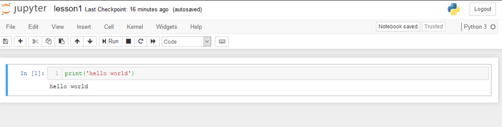
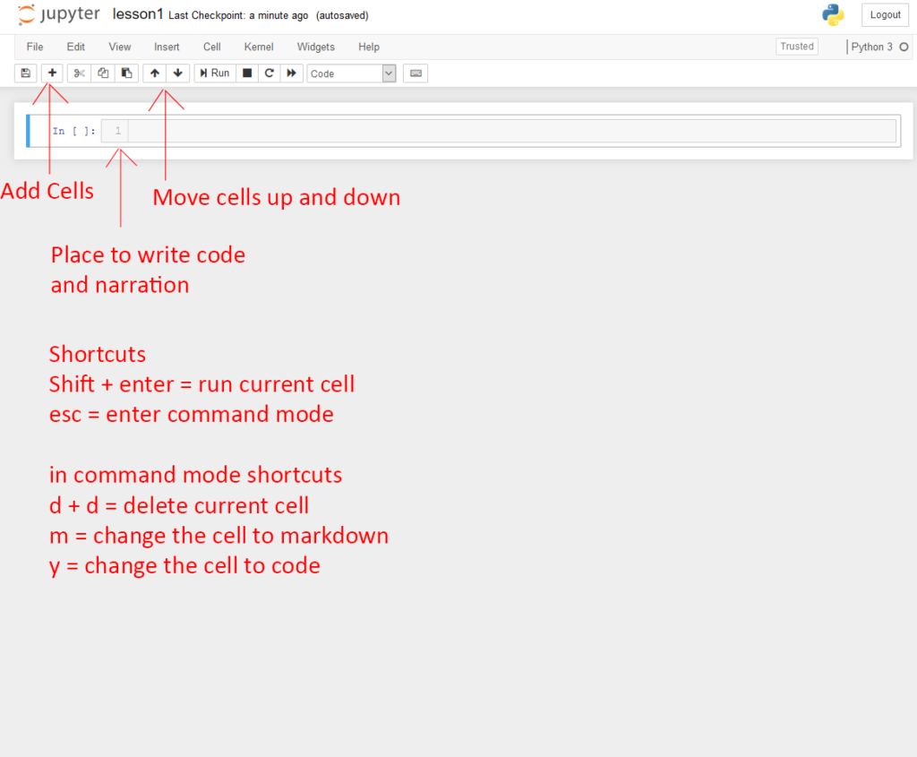
மேலே உள்ள screenshot இல் Jupyter interface பற்றி தெளிவாக ஆங்கிலத்தில் குறிப்பிடப்பட்டுள்ளது. இதில் உள்ள Shortcut களும் ஆங்கிலத்தில் குறிப்பிடப்பட்டுள்ளது. 

நாம் இப்பொழுது ஒரு Basic Python program ஐ பார்ப்போம். கீழே உள்ள Code ஐ Copy செய்து Cell இல் Paste செய்யுங்கள். 

print('hello world')

நமக்கு கீழே உள்ள Screenshot போல output கிடைக்கும்.

சரி நண்பர்களே அடுத்த post இல் variables, functions, machine learning specific packages numPy, Pandas, Sklearn, Tensorflow, Kares, பற்றி பார்போம்.

நீங்கள் இந்த post ஐ ஆங்கிலத்தில் படிக்க விரும்பினால் கீழே உள்ள Link ஐ Click செய்யவும்.

நன்றி நண்பர்களே 

இந்த Post இல் பிழை இருந்தால் மன்னிக்கவும்.